Problem Overview
The superstore is prepping for a high-stakes, year-end marketing campaign, a limited time Gold Membership offer: 20% off all purchases for just $499 (usually $999). But this offer isn’t for everyone, only existing customers, and the plan is to reach them through phone calls.
Now here’s the challenge: calling every customer eats up time, resources, and money. And not everyone will say yes.
So instead of calling blindly, the business wants to know:
“Can we predict the kind of customers who are more likely to say yes to the offer and focus our efforts on them?”
Using past campaign data, i want to understand which customer traits lead to a positive response, and build a predictive model that helps the business call only the right people.
Project Objectives
🔹 Predict the likelihood of a customer responding positively
🔹 Identify the key factors that influence customer response

 View the project notebook on GitHub
You can also view more project on my portfolio here, i also write content on Data Analytic/Data Science, visit my Blog post here
Exploratory Data Analysis
For this project, I used the Superstore Marketing Campaign Dataset from Kaggle, which contains customer-level data including demographics, product purchases, web interactions, and campaign responses. You can view the analysis notebook here on Kaggle
The original dataset had 2,240 rows and 22 columns. To begin the analysis, I performed a quick quality check to identify any missing values or data inconsistencies. It showed that only the Income column had missing values, 24 rows in total. Since the number was small relative to the dataset size, I chose to drop those rows to keep things simple and avoid adding noise through imputation. After this cleanup, the dataset was reduced to 2,216 rows, with no missing values across any other columns. This ensured we had a clean dataset to proceed with meaningful analysis and model building.
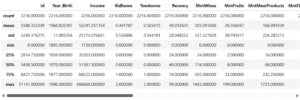
From the summary, we saw that the average income of customers is around $52,000, but there’s a huge spread, with some incomes as high as $666,666, which is likely an outlier. Most customers were born between the 1950s and late 1970s, with the average birth year around 1968. Also, the average number of kids and teenagers at home is low (less than 1 each), which suggests that most customers probably don’t have children living with them. For purchases, the average spending is highest on wine and meat products. This snapshot gave us a first sense of data distribution, potential outliers, and where we might need to dig deeper during EDA.
Please visit Github to view the analysis codes and outputs.
By the way i recently did an analysis on the Profitability Analysis of a retail Ads Campaign, check it out here
Let’s check the distribution in details;
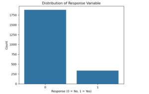
Next, i checked the distribution of the target variable the “Response” column. From the chart, it was clear that most customers didn’t respond to the marketing campaign. Out of over 2,200 people, about 1,800 said “No” while only around 300 said “Yes”. This means the data is imbalanced, and we have to be careful when building a model because predicting “No” every time would still look accurate, but it wouldn’t help the business target the right people.
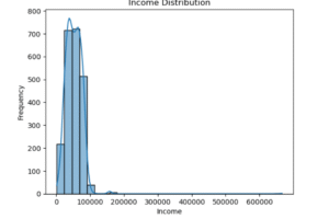
Next, I explored the “Income” column. The income distribution showed that most customers earned between $25,000 and $80,000. There were also a few people earning above $100,000, and some even close to $600,000. Those are outliers. It’s something to watch because extreme values like that can affect analysis and model performance. Depending on what the business wants, we might need to cap or remove them.
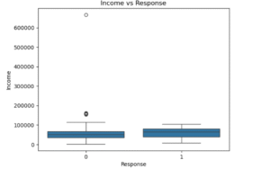
Then I looked at income against the response using a box plot. It showed that people who responded “Yes” had a slightly higher average income compared to those who didn’t. Also, the income spread was tighter for responders, while non-responders had more low-income customers and more variation. This could mean that people with higher income are more likely to respond, which might be useful when deciding who to focus on in future campaigns.
Data Preparation
At this stage, I focused on data preparation to create meaningful features for the modeling phase. Starting with the original dataset, I created a copy called data_subset for transformation. To better represent household dynamics, I combined the Kidhome and Teenhome columns into a new feature TotalChildren, and from there, derived HouseholdSize and IncomePerPerson for more accurate per capita metrics.
Next, I aggregated spending behavior across six product categories (like wines, meats, and gold products) into a single TotalSpent feature. From this, I calculated each product’s spending ratio relative to the total spend, such as MntWines_Ratio and MntMeatProducts_Ratio, to understand customer preferences in proportion.
Also, I aggregated purchase channels into TotalPurchases, OnlinePurchases, and OfflinePurchases, then derived a DealPurchaseRatio to capture how often customers buy via deals. I also calculated customer tenure by converting the Dt_Customer column into a TenureDays and TenureMonths variable, based on the most recent join date.
To simplify categorical variables, I grouped Marital_Status into broader categories like “Partnered”, “Single”, and “Other”, and encoded education levels into a binary variable, postgraduates as 1 and undergraduates as 0. After creating these features, I dropped redundant or transformed columns such as Id, Year_Birth, Education, and individual purchase method columns.
The updated dataset now contains 28 refined features that reflect spending behavior, household composition, purchasing habits, and tenure, ideal for feeding into a predictive model.
View the project notebook on GitHub
Let’s take a look at the transformed dataset summary!!!
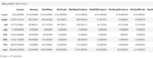
After cleaning and transforming the dataset, I noticed the stats became more reliable and usable for modeling.
Logistic regression model result
Our model achieved an accuracy score of 86.77%, which means it correctly predicted customer responses in about 87 out of every 100 cases. You can check the full model result and code on my GitHub. However, accuracy alone doesn’t tell the full story, especially for imbalanced data like this. Looking at the classification report, the model performed very well at identifying those who will not respond to the campaign (precision = 90%, recall = 95%). But it struggled to identify those who will respond, with a lower precision (59%) and recall (39%). This suggests the model is more confident in predicting non-responders but less reliable when flagging potential responders. For campaign planning, this means while we can trust who not to target, we need to improve the model further to better catch more likely responders without missing them.
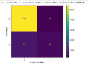
The confusion matrix shows that the model predicted 538 true negatives, people correctly identified as non-responders and 39 true positives, meaning actual responders were correctly flagged. However, it also made 27 false positive errors (people predicted to respond but didn’t) and 61 false negatives (missed actual responders). This supports what we saw earlier: the model is better at spotting non-responders than responders, which is good for avoiding wasted campaign efforts but might cause us to miss some potential conversions.
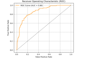
The ROC Curve shows an AUC of 0.86, which means the model does a great job at distinguishing between responders and non-responders. A perfect model scores 1.0, and anything above 0.80 is considered strong, so this gives confidence that the model is reliably ranking customers based on their likelihood to respond.
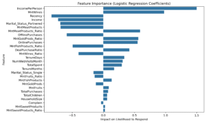
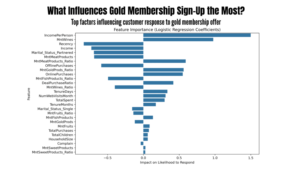
The visual above shows the top features influencing the campaign response, based on their logistic regression coefficients. Features with positive values (like IncomePerPerson, MntWines, and DealPurchaseRatio) increase the likelihood of a customer responding. On the other hand, features with negative values (such as Recency, Income, and MntMeatProducts) reduce the likelihood of response.
Lastly, I want to plot the most influential feature against the target variable to visualize predicted probabilities and their confidence.
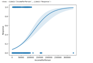
This chart clearly shows that as an individual’s income per household member goes up, their chances of responding to the offer increase significantly. We see a big jump in responses, especially from households where the income per person is around $75,000 to $200,000. This tells us that focusing our marketing on these segments will likely lead to much better results and more efficient spending.
This will gives the marketing team insight into what characteristics define likely responders, especially income patterns, wine spending, and digital engagement.
KEY FINDING
-
High Accuracy but Class Imbalance Concerns
The model achieved an accuracy of 86.8%, which may seem impressive at first glance. However, deeper evaluation shows it performs much better at predicting non-responders (class 0) than responders (class 1).-
Precision for responders is 0.59 and recall is only 0.39, meaning many actual responders are not being correctly identified.
-
Confusion matrix reveals 538 true negatives but only 39 true positives, with 61 responders missed by the model.
-
-
Model Has Strong Predictive Power
The ROC AUC score is 0.86, suggesting good discrimination between the two classes overall, the model can separate responders from non-responders quite well. -
Income and Product Preferences Drive Response
From the feature importance chart:-
Positive drivers of response:
IncomePerPerson,MntWines,MntMeatProducts_Ratio, andOnlinePurchases. -
Negative drivers:
Recency(recent purchases),Income, and beingPartneredare associated with a lower likelihood to respond.
-
Business Insight
The model tells us that high-value customers who purchase more wines and meat, shop online often, and have higher per-person income are more likely to respond to marketing campaigns. However, the current model struggles to identify all potential responders, which could lead to missed marketing opportunities and on the other hand, it help not to waste resources.
Also, recency is negatively associated, meaning those who haven’t purchased in a while may actually be more responsive, that’s a pattern worth exploring.
Recommendation
-
Marketing teams should prioritize calling customers identified as likely responders through the model
With an accuracy of 86.7% and an AUC of 0.86, the predictive model is a reliable tool for reducing unnecessary calls. Instead of reaching out to everyone, agents can use the model’s output to contact only those most likely to accept the offer. This allows the team to spend less time on cold leads and more time on warm ones, ultimately lowering campaign costs and improving outcomes. -
Sales representatives should highlight premium categories like wine, meat, and sweets during calls
These product categories had the strongest influence on whether a customer said yes to the offer. If a customer has consistently spent on these items, reps should use that behavior in the conversation, for example: “Since you’ve enjoyed our fine wine and gourmet selections, you’ll get even more value with the gold membership’s discount”. -
Campaign planners should consider IncomePerPerson when deciding which segments to approach
While total income didn’t tell us much, IncomePerPerson, the income divided across household members, was a meaningful predictor. This tells us that a household with fewer people and decent income is more likely to respond positively. Prioritizing these segments can lead to better conversion with fewer wasted efforts. -
Retention specialists should re-engage customers who haven’t purchased recently
Interestingly, customers with longer gaps since their last purchase were more open to the offer. This presents an opportunity to reconnect with dormant customers. Scripts can be tailored to say, “We’ve missed you, here’s a special membership to welcome you back with exclusive year-end benefits”.